The Sigmoid Function: From ‘e’ to Neural Networks

Welcome back!

We recently discussed backpropagation, and I hope you now have an idea of what backpropagation is and how it actually works.

Let’s continue the deep learning journey.

Even though we apply the backpropagation algorithm to a neural network, we still have some problems, and vanishing gradients is one of them.

While I was learning about vanishing gradients, I came across the sigmoid function.

We all know that it is used in logistic regression, where we apply the sigmoid function to a value to obtain an output between 0 and 1.

Now, here in neural networks, it can be used as an activation function.

What I know about sigmoid is the equation we have and its usage in logistic regression and neural networks.

I was curious about how we get this equation and the story behind it.

In this blog, let’s see how we get to the sigmoid equation.

By the way, if you haven’t read Part 3 of the backpropagation series, you can read it here.

···

How Do We Actually Use Sigmoid?

We already know the equation of the sigmoid function.

\sigma(x) = \frac{1}{1 + e^{-x}}

Before we proceed, let’s see how we use it in logistic regression.

For example, we want to predict whether a student will pass or fail based on the number of hours they studied.

We are using the logistic regression model here.

First, it calculates a score

Let’s say the score for a student is:

This score is not a probability.

It is just the linear combination of parameters.

Now we pass it through the sigmoid function:

\sigma(z) = \frac{1}{1 + e^{-z}}

we get,

\sigma(2) = \frac{1}{1 + e^{-2}} \approx 0.88

The sigmoid function always produces an output between 0 and 1.

Here the output is approximately 0.88 or 88%.

In logistic regression, this can be interpreted as an 88% probability of the student passing the exam.

We can then use a threshold, such as 0.5, to make the final classification.

In short, the flow can be like

\text{Score} \rightarrow \text{Sigmoid} \rightarrow \text{Probability} \rightarrow \text{Class}

That’s how we commonly use the sigmoid function in logistic regression.

But What Is This “e”?

Now, let’s once again look at the sigmoid equation.

\sigma(z) = \frac{1}{1 + e^{-z}}

The first thing we notice is the e.

We know that it is a mathematical constant and its value is

e \approx 2.71828

But what exactly is ‘e’?

Why is this number present in the sigmoid equation?

Let’s take a step back and understand where this number comes from.

One thing is that here we are not trying to discover ‘e’, but the goal is to understand the significance of ‘e’ and see where it naturally appears.

Now let’s go to the bank and see what we can observe.

Let’s Start with a Simple Bank Example

Imagine we deposited Rs.100 into a bank account.

Let’s say the bank is giving us a 100% annual interest rate.

If the bank adds the entire year’s interest at the end of the year, we earn Rs.100 in interest.

So after one year, we have

100 + 100 = 200

We can also write it as

100(1 + 1) = 200

Rs.100 became Rs.200 after one year.

But now let’s change one thing.

What if the bank doesn’t wait until the end of the year to add the interest?

What if it adds the interest twice a year?

The annual interest rate is still 100%.

But now the year is divided into two periods.

So for each six-month period we get half of the annual interest rate:

\frac{1}{2} = 0.5 = 50\%

During the first six months, we get

100\left(1 + \frac{1}{2}\right) = 150

After six months, we have Rs.150.

During the next six months, the interest is calculated on this new amount

150\left(1 + \frac{1}{2}\right) = 225

Then we have

100\left(1 + \frac{1}{2}\right)^2 = 225

Why did we get Rs.225 instead of Rs.200?

Because the interest earned during the first six months also earned interest during the second six months.

In simple terms we can say

‘interest earns interest’

This is the basic idea behind compound interest.

What Happens When We Compound More Frequently?

Now let’s make the compounding more frequent.

If we compound four times a year:

100\left(1 + \frac{1}{4}\right)^4 \approx 244.14

If we compound 12 times a year:

100\left(1 + \frac{1}{12}\right)^{12} \approx 261.30

If we compound every day:

100\left(1 + \frac{1}{365}\right)^{365} \approx 271.46

Observe the pattern.

As we increase the number of compounding periods, the final amount keeps increasing.

The reason is that growth is being applied repeatedly to an amount that has already increased.

Where Does e Come From?

The Rs.100 is not the important part here.

Let’s remove it and look at the growth factor:

\left(1 + \frac{1}{n}\right)^n

Here, ‘n’ represents the number of times we compound during the year.

For example:

\left(1 + \frac{1}{1}\right)^1 = 2

\left(1 + \frac{1}{2}\right)^2 = 2.25

\left(1 + \frac{1}{4}\right)^4 \approx 2.4414

\left(1 + \frac{1}{12}\right)^{12} \approx 2.613

\left(1 + \frac{1}{365}\right)^{365} \approx 2.7146

As we make the compounding more and more frequent, the value gets closer and closer to

2.71828\ldots

This number is called ‘e’

e \approx 2.71828

Mathematically, we can express this idea using a limit

e = \lim_{n \rightarrow \infty} \left(1 + \frac{1}{n}\right)^n

The notation may look complex, but the idea is simple.

Here, we are asking:

“What value does this expression approach as ‘n’ becomes larger and larger?”

As ‘n’ increases:

\left(1 + \frac{1}{n}\right)^n

gets closer and closer to:

2.71828\ldots

That limiting value is ‘e’.

So, What Does the Bank Have to Do with Sigmoid?

But why are we talking about this and what does this bank account have to do with sigmoid.

This example isn’t to explain compound interest, but it gives us an intuition for where ‘e’ naturally appears.

The important idea here is repeated growth.

When growth is repeatedly applied to an amount that has already grown, we get a compounding process.

And when that process happens again and again more frequently, the number ‘e’ naturally appears.

So instead of simply memorizing that

e \approx 2.71828

we now have some intuition behind it.

The Special Property of e

From the bank example, we observed that ‘e’ naturally appears when we look at repeated growth and continuous compounding.

But ‘e’ is more than just a number that appears in compound interest.

It has a very special property when we look at it through calculus.

Let’s consider the exponential function

If we differentiate this function, we get

\frac{dy}{dx}=e^x

This formula we already know.

But what does the derivative tell us?

We already know that it tells us the rate of change of a function.

For example, if we have

its derivative is

\frac{dy}{dx}=2x

This means that the rate at which x2 changes depends on the value of x.

At x=1:

\frac{dy}{dx}=2(1)=2

At x=3:

\frac{dy}{dx}=2(3)=6

So, for x2, the function and its rate of change are different.

Now let’s look at ex.

For

we have

\frac{dy}{dx}=e^x

This means that the rate of change of ex is equal to its current value.

Let’s look at some values.

When x=0

and

\frac{dy}{dx}=1

When x=1

e^1\approx2.718

and

\frac{dy}{dx}\approx2.718

When x=2

e^2\approx7.389

and

\frac{dy}{dx}\approx7.389

So, here we can say that

Rate of change = Current value

This is one of the most important properties of the exponential function with base e.

Why Is the Derivative of ex Equal to ex?

We now have an idea of an important property of ‘e’ in calculus.

\frac{d}{dx}e^x=e^x

We just discussed what it is but let’s see why does this happen?

If you already know why

\frac{d}{dx}e^x=e^x

then use this section for quick revision as we connect it back to the sigmoid function.

Starting with a General Exponential

First let’s consider a general exponential function.

Here, z is the base and x is the exponent.

2^x,\qquad 3^x,\qquad 5^x,\qquad 10^x

are all examples of this form.

Now let’s see what happens when we differentiate zx

We have,

\frac{dy}{dx} = \lim_{h\to0} \frac{z^{x+h}-z^x}{h}

Using the exponent rule we get

z^{x+h}=z^xz^h

Therefore

\frac{dy}{dx} = \lim_{h\to0} \frac{z^xz^h-z^x}{h}

Now notice that zx appears in both terms in the numerator.

We can factor it out

\frac{dy}{dx} = \lim_{h\to0} z^x\frac{z^h-1}{h}

Here zx does not depend on h, so we can take it outside the limit

\frac{dy}{dx} = z^x \lim_{h\to0} \frac{z^h-1}{h}

And this is where things get interesting.

Our result is

\frac{dy}{dx} = z^x \lim_{h\to0} \frac{z^h-1}{h}

Look at the two parts separately.

The first part is

That is our original exponential function.

The second part is

\lim_{h\to0} \frac{z^h-1}{h}

We can see that there is no ‘x’ in this expression.

It depends on the base ‘z’, but not on ‘x’.

This means, for any value of ‘z’, this entire limit is just a constant.

Let’s call this constant ‘C’.

C= \lim_{h\to0} \frac{z^h-1}{h}

Therefore we can write it as,

\frac{d}{dx}z^x=Cz^x

This tells us something important.

When we differentiate an exponential function, we get the original exponential function, multiplied by a constant.

In other way,

\text{Derivative of }z^x = \text{constant}\times z^x

The Constant Depends on the Base

Now let’s take an example of exponential function:

From our result, we have

\frac{d}{dx}3^x=C3^x

For z=3, the constant is

C= \lim_{h\to0} \frac{3^h-1}{h}

Now we need to find the value of this limit.

Let’s understand this in intuitive way.

For the base 3, the value of the constant is approximately

C\approx1.0986

Therefore,

\frac{d}{dx}3^x \approx 1.0986(3^x)

Let’s see what this tells us by using at different ‘x’ values.

When

we have

the rate of change here is approximately

1.0986(1)=1.0986

When

we get

The rate of change is

1.0986(3)\approx3.2958

And when

we have

The rate of change is approximately

1.0986(9)\approx9.8874

We can see that the derivative is not exactly equal to 3x.

Instead, we got

\frac{d}{dx}3^x \approx 1.0986(3^x)

The function and its rate of change have the same exponential shape, but the rate of change is scaled by a constant.

Finding the Special Base

Now, we know that

\frac{d}{dx}z^x=Cz^x

The value of ‘C’ depended on the base.

For 3x,

C\approx1.0986

Ok but what if we could find a base for which C is exactly 1?

Do we have any number?

If yes, then we get

Our derivative would become

\frac{d}{dx}z^x=z^x

In other words, we can say that the function would be exactly equal to its own derivative.

So, now we are looking for a base z that satisfies

\lim_{h\to0} \frac{z^h-1}{h}=1

There is one particular positive number that satisfies this condition and you all know what’s that number is.

We call this number

and its numerical value is

e\approx2.71828

For this particular base, the constant becomes

Therefore,

\frac{d}{dx}e^x = 1\cdot e^x

which gives us

\frac{d}{dx}e^x=e^x

···

So What Did We Actually Discover?

We started with a general exponential function

Using the definition of a derivative, we found

\frac{d}{dx}z^x = z^x \lim_{h\to0} \frac{z^h-1}{h}

We then observed that the limit is simply a constant that depends on the base.

Then we have written it as

\frac{d}{dx}z^x=Cz^x

Then we asked:

Is there a base for which C=1?

The answer is yes.

That special base is e.

Therefore,

\frac{d}{dx}e^x=e^x

Now we have an idea of how we got the derivative.

In the earlier bank example, ‘e’ appeared through repeated growth and continuous compounding.

Now, through calculus, we have seen another special property of the same number

\frac{d}{dx}e^x=e^x

In simple words, we can say that ex grows at a rate equal to its current value.

Now, Let’s Return to Sigmoid

Let’s once again look at the sigmoid equation.

\sigma(x)=\frac{1}{1+e^{-x}}

Now we have some idea of what ‘e’ actually is.

Now we focus on the whole equation.

The question here is why does the sigmoid function is in this particular form?

To understand this we should go back to logistic regression.

We started with a raw score

‘z’ can be any real number.

But for classification, we wanted to interpret the model’s output as a probability.

A probability must lie between 0 and 1

$0<p<1$

So we want to transform any value of ‘z’ into a value between 0 and 1.

In other words, we want something that can receive

z\in(-\infty,\infty)

and produce:

p\in(0,1)

Building a Function That Outputs Between 0 and 1

Now, the task is to construct such transformation.

But how can we do that?

Let’s start with a very simple observation.

Suppose we have a number greater than 1.

For example

If we take its reciprocal, we get

\frac{1}{5}=0.2

which is between 0 and 1.

The same idea works for any numbers greater than 1

\frac{1}{2}=0.5

\frac{1}{10}=0.1

\frac{1}{100}=0.01

Here we can notice that

then

0 < \frac{1}{A} < 1

This gives us a simple idea.

If we can have a quantity that is always greater than 1, then taking its reciprocal will automatically give us a value between 0 and 1.

And that is exactly the range we want for a probability.

However, there is one more thing we need.

We do not want to use a fixed number such as 5 in the denominator.

because that always give us the same output.

Our output should change when the input ‘x’ changes.

For example, we want a positive input to produce a larger probability, while a negative input should produce a smaller probability.

So, we need a quantity that changes with x.

Now e Enters the Picture

You are right. It’s time for ‘e’ to enter.

This is where the exponential function we just learned about becomes useful.

Exponential functions are always positive, which means

for every real value of x.

For example:

e^{-2}\approx0.1353

e^2\approx7.389

Whether the x is negative, zero, or positive, ex never becomes negative or zero.

But the sigmoid equation contains e-x.

Till here we only discussed about ex.

So let’s first see what a negative exponent means.

We already know what a positive exponent means.

For example:

e^2=e\times e

and:

e^3=e\times e\times e

A negative exponent represents the reciprocal of the corresponding positive exponent.

For example:

e^{-1}=\frac{1}{e}

Similarly

e^{-2}=\frac{1}{e^2}

and

e^{-3}=\frac{1}{e^3}

In general, we can write as

e^{-x}=\frac{1}{e^x}

So, e-x is not a completely different function.

It is simply the reciprocal of ex.

Now we can use what we already know about ex.

Since:

its reciprocal is also positive

\frac{1}{e^x}>0

and because

e^{-x}=\frac{1}{e^x}

we get

for every real value of x.

This is important because it gives us exactly the kind of quantity we need.

If e-x is always positive, then adding 1 gives us a quantity that is always greater than 1

1+e^{-x}>1

And now we can use our reciprocal idea.

If a number is greater than 1, its reciprocal lies between 0 and 1

0<\frac{1}{1+e^{-x}}<1

Now we have a function whose output is always between 0 and 1.

The expression we just got is

\frac{1}{1+e^{-x}}

and this is exactly the sigmoid function we started with

\sigma(x)=\frac{1}{1+e^{-x}}

So instead of looking at the sigmoid equation as a formula, now we can understand the intuition behind its structure.

We wanted the output to lie between 0 and 1.

We observed that the reciprocal of a number greater than 1 lies between 0 and 1.

As e-x is always positive, we used it to construct a quantity greater than 1

1+e^{-x}>1

Taking its reciprocal gave us

\sigma(x)=\frac{1}{1+e^{-x}}

This gave us the range we wanted.

But does this equation actually behave the way we expected it to do?

Here, our goal is to understand the intuition behind the structure of the sigmoid function.

There are other functions that can map values to the range 0 to 1, and why logistic regression uses sigmoid is related to odds and log-odds, a topic which we will explore in future blogs.

Does the Sigmoid Behave the Way We Expected?

Let’s test on few values.

First, let’s consider

Substituting into the sigmoid function:

\sigma(0)=\frac{1}{1+e^{-0}}

we get

\sigma(0)=\frac{1}{1+1}=0.5

When the input is 0, the sigmoid gives us exactly 0.5.

Now let’s take a positive number

then

\sigma(2)=\frac{1}{1+e^{-2}}

We already seen

e^{-2}\approx0.1353

which gives

\sigma(2) = \frac{1}{1+0.1353} = \frac{1}{1.1353} \approx 0.881

The sigmoid converted the input 2 into approximately 0.881 or 88.1%.

Now let’s see what happens when the input is a negative number.

Consider

Then

\sigma(-2) = \frac{1}{1+e^{-(-2)}}

\sigma(-2) = \frac{1}{1+e^2}

We know

e^2\approx7.389

Finally we get

\begin{aligned} \sigma(-2) &=\frac{1}{1+7.389}\\ &=\frac{1}{8.389}\\ &\approx0.119 \end{aligned}

So the sigmoid converted the input -2 into approximately 0.119 or 11.9%.

Now we can see how the sigmoid behaves.

For a negative input:

x=-2 \quad\longrightarrow\quad \sigma(x)\approx0.119

For zero:

x=0 \quad\longrightarrow\quad \sigma(x)=0.5

For a positive input:

x=2 \quad\longrightarrow\quad \sigma(x)\approx0.881

So as x increases, the sigmoid output moves from values close to 0, passes through 0.5 and moves toward 1.

In the extreme cases:

x\rightarrow-\infty \quad\Longrightarrow\quad \sigma(x)\rightarrow0

and

x\rightarrow+\infty \quad\Longrightarrow\quad \sigma(x)\rightarrow1

This is exactly the behavior we wanted from a function that transforms any real number into something between 0 and 1.

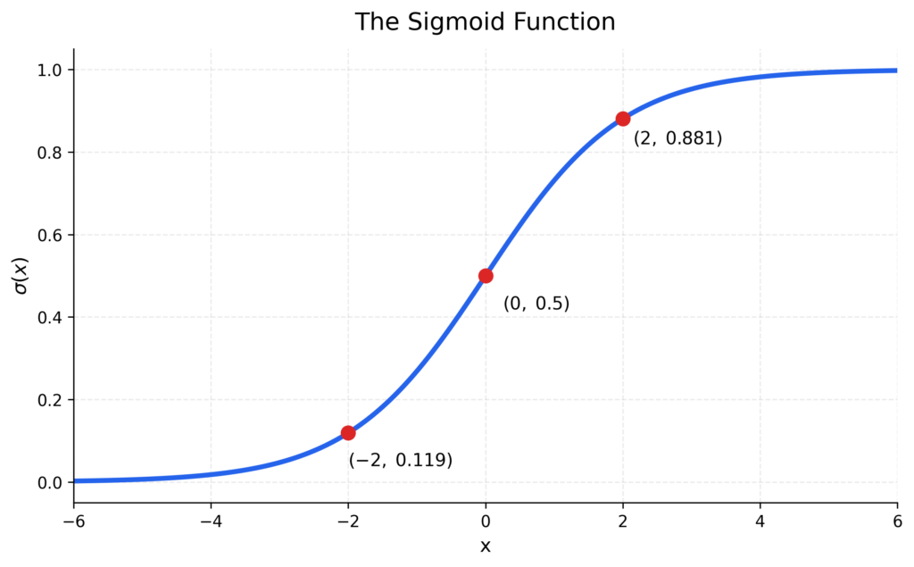
Now we have an idea of how we got the equation of the sigmoid function.

If you remember, in my recent blogs, when we discussed backpropagation and neural networks in general, we talked about activation functions and why they are important.

We used the ReLU activation function to understand those concepts.

Now, we can also use sigmoid as an activation function.

But if we use sigmoid as an activation function, there is one more thing we need to know.

During the backward pass, we already know that the network calculates gradients using derivatives.

So, if sigmoid is part of the network, we need to differentiate it as well.

Now let’s focus only on deriving the derivative of the sigmoid function step by step.

\sigma(x)=\frac{1}{1+e^{-x}}

Instead of carrying the exponential term throughout calculations, we can simply use the sigmoid output itself.

This is the derivative we use whenever sigmoid appears in the gradient calculations of a neural network.

···

Summary

In the upcoming blogs, we are going to discuss topics like vanishing gradients and exploding gradients.

As we explore these topics, we will come across the sigmoid function, and we will also need its derivative.

If we derive the sigmoid function and its derivative in those blogs, the discussion could become long, and we may lose focus on the actual concept that we are trying to understand.

It would also be better to have an idea of where the sigmoid function and its derivative come from before using them in further concepts.

We first started with the bank example to see how e appears. We then learned about its important property in calculus and, using these ideas, gradually built the sigmoid equation.

We saw how this equation is used in logistic regression and neural networks, and we also derived its derivative.

Now, when we move on to the upcoming topics, we already have this foundation which will be useful for us.

I hope you found this blog helpful in understanding a concept that we frequently use.

If you have any questions or suggestions for improvement, feel free to share them in the comments on LinkedIn.

And if you haven’t read my latest blog series on backpropagation yet, you can read it here.

Sometimes, moving forward means going back and understanding the basics.

Thanks for reading!

···

How Do We Actually Use Sigmoid?

But What Is This “e”?

Let’s Start with a Simple Bank Example

What Happens When We Compound More Frequently?

Where Does e Come From?

So, What Does the Bank Have to Do with Sigmoid?

The Special Property of e

Why Is the Derivative of ex Equal to ex?

Starting with a General Exponential

Finding the Special Base

So What Did We Actually Discover?

Now, Let’s Return to Sigmoid

Building a Function That Outputs Between 0 and 1

Now e Enters the Picture

Does the Sigmoid Behave the Way We Expected?

Summary

DuckDB and the changing physics of analytics

The Sound of the Silenced: Inside the ten-year global fight to keep the internet on

Post Comment Cancel reply